Titanic: Getting Started With R - Part 3: Decision Trees

Tutorial index

Last lesson we sliced and diced the data to try and find subsets of the passengers that were more, or less, likely to survive the disaster. We climbed up the leaderboard a great deal, but it took a lot of effort to get there. To find more fine-grained subsets with predictive ability would require a lot of time to adjust our bin sizes and look at the interaction of many different variables. Luckily there is a simple and elegant algorithm that can do this work for us. Today we’re going to use machine learning to build decision trees to do the heavy lifting for us.

Decision trees have a number of advantages. They are what’s known as a glass-box model, after the model has found the patterns in the data you can see exactly what decisions will be made for unseen data that you want to predict. They are also intuitive and can be read by people with little experience in machine learning after a brief explanation. Finally, they are the basis for some of the most powerful and popular machine learning algorithms.

I won’t get into the mathematics here, but conceptually, the algorithm starts with all of the data at the root node (drawn at the top) and scans all of the variables for the best one to split on. The way it measures this is to make the split on the variable that results in the most pure nodes below it, ie with either the most 1’s or the most 0’9s in the resulting buckets. But let’s look at something more familiar to get the idea. Here we draw a decision tree for only the gender variable, and some familiar numbers jump out:

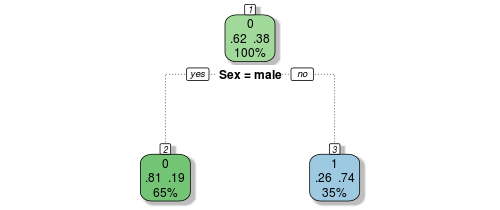
Let’s decode the numbers shown on this new representation of our original manual gender-based model. The root node, at the top, shows our tutorial one insights, 62% of passengers die, while 38% survive. The number above these proportions indicates the way that the node is voting (recall we decided at this top level that everyone would die, or be coded as zero) and the number below indicates the proportion of the population that resides in this node, or bucket (here at the top level it is everyone, 100%).

So far, so good. Now let’s travel down the tree branches to the next nodes down the tree. If the passenger was a male, indicated by the boolean choice below the node, you move left, and if female, right. The survival proportions exactly match those we found in tutorial two through our proportion tables. If the passenger was male, only 19% survive, so the bucket votes that everyone here (65% of passengers) perish, while the female bucket votes in the opposite manner, most of them survive as we saw before. In fact, the above decision tree is an exact representation of our gender model from last lesson.

The final nodes at the bottom of the decision tree are known as terminal nodes, or sometimes as leaf nodes. After all the boolean choices have been made for a given passenger, they will end up in one of the leaf nodes, and the majority vote of all passengers in that bucket determine how we will predict for new passengers with unknown fates.

But you can keep going, and this is what I alluded to at the end of the last lesson. We can grow this tree until every passenger is classified and all the nodes are marked with either 0% or 100% chance of survival… All that chopping and comparing of subsets is taken care of for us in the blink of an eye!

Decision trees do have some drawbacks though, they are greedy. They make the decision on the current node which appear to be the best at the time, but are unable to change their minds as they grow new nodes. Perhaps a better, more pure, tree would have been grown if the gender split occurred later? It is really hard to tell, there are a huge number of decisions that could be made, and exploring every possible version of a tree is extremely computationally expensive. This is why the greedy algorithm is used.

As an example, imagine a cashier in a make-believe world with a currency including 25c, 15c and 1c coins. The cashier must make change for 30c using the smallest number of coins possible. A greedy algorithm would start with the coin that leaves the smallest amount of change left to pay:

• Greedy: 25 + 1 + 1 + 1 + 1 + 1 = 30c, with 6 coins
• Optimal: 15 + 15 = 30c, with 2 coins

Clearly the greedy cashier algorithm failed to find the best solution here, and the same is true with decision trees. Though they usually do a great job given their speed and the other advantages we already mentioned, the optimal solution is not guaranteed. Decision trees are also prone to overfitting which requires us to use caution with how deep we grow them as we’ll see later.

So, let’s get started with our first real algo! Now we start to open up the power of R: its packages. R is extremely extensible, you’d be hard pressed to find a package that doesn’t automatically do what you need. There’s thousands of options out there written by people who needed the functionality and published their work. You can easily add these packages within R with just a couple of commands.

The one we’ll need for this lesson comes with R. It’s called rpart for “Recursive Partitioning and Regression Trees” and uses the CART decision tree algorithm. While rpart comes with base R, you still need to import the functionality each time you want to use it. Go ahead:

> library(rpart)

Now let’s build our first model. Let’s take a quick review of the possible variables we could look at. Last time we used aggregate and proportion tables to compare gender, age, class and fare. But we never did investigate SibSp, Parch or Embarked. The remaining variables of passenger name, ticket number and cabin number are all unique identifiers for now; they don’t give any new subsets that would be interesting for a decision tree. So let’s build a tree off everything else.

The format of the rpart command works similarly to the aggregate function we used in tutorial 2. You feed it the equation, headed up by the variable of interest and followed by the variables used for prediction. You then point it at the data, and for now, follow with the type of prediction you want to run (see ?rpart for more info). If you wanted to predict a continuous variable, such as age, you may use method="anova". This would run generate decimal quantities for you. But here, we just want a one or a zero, so method="class" is appropriate:

> fit <- rpart(Survived ~ Pclass + Sex + Age + SibSp + Parch + Fare + Embarked,
               data=train,
               method="class")

Let’s examine the tree. There are a lot of ways to do this, and the built-in version requires running

> plot(fit)
> text(fit)

Hmm, not very pretty or insightful. To get some more informative graphics, you will need to install some external packages. As I mentioned, tons of world-class developers donate their time and energy to the R project by contributing powerful packages to CRAN, free of charge. You can install them from within R using install.packages(), and load them as before with library(). Here are the ones we need for some better graphics for rpart:

> install.packages('rattle')
> install.packages('rpart.plot')
> install.packages('RColorBrewer')
> library(rattle)
> library(rpart.plot)
> library(RColorBrewer)

Let’s try rendering this tree a bit nicer with fancyRpartPlot (of course).

> fancyRpartPlot(fit)

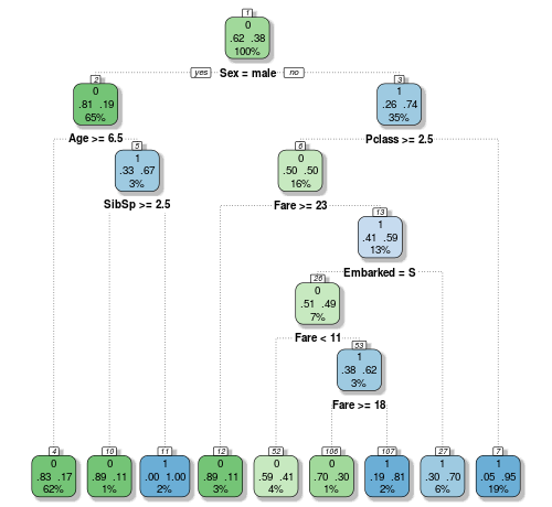
Okay, now we’ve got somewhere readable. The decisions that have been found go a lot deeper than what we saw last time when we looked for them manually. Decisions have been found for the SipSp variable, as well as the port of embarkation one that we didn’t even look at. And on the male side, the kids younger than 6 years old have a better chance of survival, even if there weren’t too many aboard. That resonates with the famous naval law we mentioned earlier. It all looks very promising, so let’s send another submission into Kaggle!

To make a prediction from this tree doesn’t require all the subsetting and overwriting we did last lesson, it’s actually a lot easier.

> Prediction <- predict(fit, test, type = "class")
> submit <- data.frame(PassengerId = test$PassengerId, Survived = Prediction)
< write.csv(submit, file = "myfirstdtree.csv", row.names = FALSE)

Here we have called rpart’s predict function. Here we point the function to the model’s fit object, which contains all of the decisions we see above, and tell it to work its magic on the test dataframe. No need to tell it which variables we originally used in the model-building phase, it automatically looks for them and will certainly let you know if something is wrong. Finally we tell it to again use the class method (for ones and zeros output) and as before write the output to a dataframe and submission file.

Let’s send it in and see how our algorithm performed!

Nice! We just jumped hundreds of spots with only an extra 0.5% increase in accuracy! Are you getting the picture here? The higher you climb in a Kaggle leaderboard, the more important these fractional percentage bumps become.

The rpart package automatically caps the depth that the tree grows by using a metric called complexity which stops the resulting model from getting too out of hand. But we already saw that a more complex model than what we made ourselves did a bit better, so why not go all out and override the defaults? Let’s do it.

You can find the default limits by typing ?rpart.control. The first one we want to unleash is the cp parameter, this is the metric that stops splits that aren’t deemed important enough. The other one we want to open up is minsplit which governs how many passengers must sit in a bucket before even looking for a split. Let’s max both out and reduce cp to zero and minsplit to 2 (no split would obviously be possible for a single passenger in a bucket):

> fit <- rpart(Survived ~ Pclass + Sex + Age + SibSp + Parch + Fare + Embarked,
               data=train,
               method="class", 
               control=rpart.control(minsplit=2, cp=0))
> fancyRpartPlot(fit)

Okay, I can’t even see what’s going on here, but with that much subsetting and mining for tiny nuggets of truth, how could we go wrong? Let’s make a sub from this model and get to the top of the leaderboard!

Even our simple gender model did better! What went wrong? Welcome to overfitting.

Overfitting is technically defined as a model that performs better on a training set than another simpler model, but does worse on unseen data, as we saw here. We went too far and grew our decision tree out to encompass massively complex rules that may not generalize to unknown passengers. Perhaps that 34 year old female in third class who paid $20.17 for a ticket from Southampton with a sister and mother aboard may have been a bit of a rare case after all.

The point of this exercise was that you must use caution with decision trees. While this particular tree may have been 100% accurate on the data that you trained it on, even a trivial tree with only one rule could beat it on unseen data. You just overfit big time!

Use caution with decision trees, and any other algorithm actually, or you can find yourself making rules from the noise you’ve mistaken for signal!

Before moving on, I encourage you to have a play with the various control parameters we saw in the rpart.control help file. Perhaps you can find a tree that does a little better by either growing it out further, or reigning it in. You can also manually trim trees in R with these commands:

> fit <- rpart(Survived ~ Pclass + Sex + Age + SibSp + Parch + Fare + Embarked,
               data=train,
               method="class",
               control=rpart.control( your controls ))
> new.fit <- prp(fit,snip=TRUE)$obj
> fancyRpartPlot(new.fit)

An interactive version of the decision tree will appear in the plot tab where you simply click on the nodes that you want to kill. Once you’re satisfied with the tree, hit “quit” and it will be stored to the new.fit object. Try to look for overly complex decisions being made, and kill the nodes that appear to go to far.

Next lesson, we will push the envelope further by introducing some feature engineering concepts. Go there now!

All code from this tutorial is available on my Github repository