Titanic: Getting Started With R - Part 1: Booting Up R

Tutorial index

Welcome to part 1 of the Getting Started With R tutorial for the Kaggle Titanic competition. This lesson will guide you through the basics of loading and navigating data in R.

Go ahead and install R (or if you’re running Linux, sudo apt-get install r-base) as well as its de facto IDE RStudio

Now head on over to Kaggle, sign-up for an account, and get the data! Here you will want to download the two datasets mentioned in the introduction, train.csv and test.csv, and save them somewhere convenient. While you’re on this page, scroll down to the variable descriptions to see what data you’ll be working with. You may wish to refer back to this as the tutorial progresses.

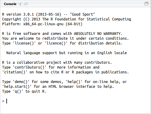
Open RStudio and you will be met with three panes. On the left is the console, this is where you enter your commands to be executed:

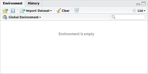
The top-right has a list of the current objects in the environment:

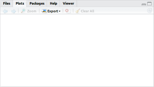
And the bottom-right has a series of tabs including your plots and help:

You can request documentation by prepending the function of interest with a question mark, for example ?table will load the help file on the table command in this help tab.

The first thing you will want to do is set your working directory. This changes the default location for all file input and output that you will do in the current session. RStudio makes this easy, simply click Session -> Set Working Directory -> Choose Directory… and navigate to where you saved your train and test sets. You should notice it has entered the command you would have typed to do this manually in the console.

While you can complete this tutorial at the command line, I would suggest creating a script to save all your hard work. This way you can easily reproduce the results or make small changes without retyping everything. Click the new document button in the top-left corner and select “R Script”. A fourth pane will now appear in the top-left. Go ahead and copy the setwd command from the console and paste it into your script. Now save the script to your working directory.

Some shortcuts to make your life a little easier. You can execute a command in the script pane by moving the cursor to that line and hitting Ctrl-Enter. Within the console, you can use the up and down arrows to find recent commands, and hitting tab will auto-complete commands and object names if possible.

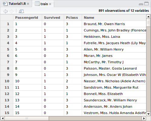
Okay, let’s load the data and have a look at it. In the top-right pane, hit “Import Dataset” and select train.csv. There shouldn’t be any need to adjust the defaults for this dataset, so simply click “Import”. For some datasets, headings or delimiters may not be automatically detected and this window would let you adjust the way it is imported. You will again see the manual command to import the dataset in the console, a new object in your environment pane, as well as a preview of the dataset in the script pane.

You may recognize the preview as being similar to a spreadsheet, the main difference is that you can only interact with it through the R programming language. You will see columns of data that match all the variables we saw on the Kaggle download page earlier. Import the test.csv dataset in the same manner. Go ahead and take a look through some of the information in both datasets before moving on. At any time during this tutorial you can preview what’s changed in your dataset by clicking the object in the explorer and the preview will open up again. It won’t refresh as you make changes though.

Copy both import commands into your script. It is also good practice to comment your code; you do this by adding the hash/pound symbol # to the beginning of any line. The purpose of code comments is simply to inform a reader, or yourself, of what the section of code is doing. In this case you may wish to add # Set working directory and import datafiles to the top of your file. You may also wish to put some additional information at the top such as your name, the date, or the overall purpose of the script.

The structure that our data is stored in is called a dataframe in R. You should notice in the object explorer the two dataframes’ dimensions. We see that there are 891 observations (rows) in the training set with 12 variables each. The test set is smaller, with only 418 passengers’ fate to predict, and only 11 variables since the “Survived” column is missing. It wouldn’t be much of a challenge if it weren’t right? That’s what we’re here to predict.

Let’s take a quick look at the structure of the dataframe, ie the types of variables that were loaded. We will use the str command for this:

> str(train)
'data.frame':    891 obs. of  12 variables:
 $ PassengerId: int  1 2 3 4 5 6 7 8 9 10 ...
 $ Survived   : int  0 1 1 1 0 0 0 0 1 1 ...
 $ Pclass     : int  3 1 3 1 3 3 1 3 3 2 ...
 $ Name       : Factor w/ 891 levels "Abbing, Mr. Anthony",..: 109 191 358 277 16 559 520 629 416 581 ...
 $ Sex        : Factor w/ 2 levels "female","male": 2 1 1 1 2 2 2 2 1 1 ...
 $ Age        : num  22 38 26 35 35 NA 54 2 27 14 ...
 $ SibSp      : int  1 1 0 1 0 0 0 3 0 1 ...
 $ Parch      : int  0 0 0 0 0 0 0 1 2 0 ...
 $ Ticket     : Factor w/ 681 levels "110152","110413",..: 525 596 662 50 473 276 86 396 345 133 ...
 $ Fare       : num  7.25 71.28 7.92 53.1 8.05 ...
 $ Cabin      : Factor w/ 148 levels "","A10","A14",..: 1 83 1 57 1 1 131 1 1 1 ...
 $ Embarked   : Factor w/ 4 levels "","C","Q","S": 4 2 4 4 4 3 4 4 4 2 ...

Let’s talk about data types we see here. An “int” is an integer which can only store whole numbers, a “num” is a numeric variable which is able to hold decimals, and a “factor” is like a category. By default, R will import all text strings as factors, and that is okay here, we can convert them back to text later if we want to manipulate them, but if the dataset has a lot of text that we know we will want to work with, we could have imported the file with

> train <- read.csv("train.csv", stringsAsFactors=FALSE)

In this case, the passengers name, their ticket number and cabin have all been imported as factors. We can see that the name variable has 891 levels, that means that no two passengers share the same factor level as that’s the total number of rows. For the other two, there are fewer levels, probably because there are missing values in there. For now, let’s leave the import command as it was, as the only factor we’ll be working with for the near-term is the gender variable, which correctly was imported as a category.

To access columns of a dataframe, there are several options, but if you want to isolate a single column of the dataframe, use the dollar sign operator. Try this is in the console: train$Survived. You should see a vector of the fates of the passengers in the training set. You can feed this vector to a function too. Let’s try table(train$Survived)

> table(train$Survived)
  0   1
549 342

The table command is one of the most basic summary statistics functions in R, it runs through the vector you gave it and simply counts the occurrence of each value in it. We see that in the training set, 342 passengers survived, while 549 died. How about a proportion? Well, we can send the output of one function into another. So now give prop.table() the output of the table function as input:

> prop.table(table(train$Survived))
        0         1
0.6161616 0.3838384

Okay, that’s a bit more readable. 38% of passengers survived the disaster in the training set. This of course means that most people aboard perished. So are you ready to make your first prediction? Since most people died in our training set, perhaps it’s a good start to assume that everyone in the test set did too? A bit morbid perhaps, but let’s break the ice (so to speak) and send in a prediction.

Some more R syntax to keep moving. The assignment operator is <- and is used to store the right hand side value to the left hand side. For instance, x <- 3 will store the value of 3 to the variable x. In some limited cases, such as passing argument values to a function signature, the equals sign is used (you’ll see this in later lessons).

Okay, so let’s add our “everyone dies” prediction to the test set dataframe. To do this we’ll need to use a new command, rep that simply repeats something by the number of times we tell it to:

> test$Survived <- rep(0, 418)

Since there was no “Survived” column in the dataframe, it will create one for us and repeat our “0” prediction 418 times, the number of rows we have. If this column already existed, it would overwrite it with the new values, so be careful! While not entirely necessary for this simple model, putting the prediction next to the existing data will help keep things in order later, so it’s a good habit to get into for more complicated predictions. If you preview the test set dataframe now, you will find our new column at the end.

We need to submit a csv file with the PassengerId as well as our Survived predictions to Kaggle. So let’s extract those two columns from the test dataframe, store them in a new container, and then send it to an output file:

> submit <- data.frame(PassengerId = test$PassengerId, Survived = test$Survived)
> write.csv(submit, file = "theyallperish.csv", row.names = FALSE)

The data.frame command has created a new dataframe with the headings consistent with those from the test set, go ahead and take a look by previewing it. The write.csv command has sent that dataframe out to a CSV file, and importantly excluded the row numbers that would cause Kaggle to reject our submission.

Okay, the file should have written to your working directory, so first make sure you can see it in your working directory and then head back to Kaggle and click “Make a submission”. You may be asked to register a team now; it’s okay if you’re planning to compete solo, every entrant needs to be part of a team, even if there’s only a single member. You can add more people later if you want to, though you cannot kick anyone out once you’ve sent in a submission.

You have 5 submissions per day in the Titanic competition; this is great news as we’ll generate a couple more in part 2! Anyhow, now that you have your team set up, either drag the csv file you just created to the yellow box on the submit page, or click the button and browse to it. Then hit submit! After the gears turn you should see something like this:

Oh wow, that was terrible! We’re close to dead last!

Relax, this tutorial was meant to get you comfortable with moving around R and RStudio. I guarantee by the time this series of lessons is done, you’ll be much closer to the other end of the board. If nothing else, we’ve noticed that we have 62% of our predictions correct. This is pretty close to the amount we should have expected from the original prop.table that we ran.

Next lesson, we will look at drilling down into the other available variables for some more insights to improve our accuracy. Go there now!

All code from this tutorial is available on my Github repository