
Armchair Particle Physicist
The Higgs Boson Machine Learning Challenge was probably the most intense competition I’ve worked on, and most likely the one I’m most proud of my solution for too. Sure, there’s a lot that I could have done better, but that’s why I work on Kaggle competitions. I want to continuously improve on how I work this ML-mojo even more effectively, and to that end I feel that I’m getting there; but still have plenty to learn. And that’s a great thing.
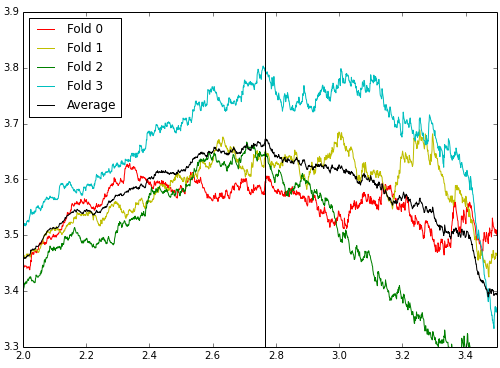
I felt the glow of the top 10 for a few days towards the end of the competition. To have hit that point on the most popular competition ever run on Kaggle (Titanic aside) is a very nice thing to have experienced, I highly recommend it. But in the end, I probably overfit to the public LB a little bit, and my time ran out before I could feel truly comfortable with my cut-off choices. Not to take away from the winners, but I also believe there was a pretty hefty element of luck in this comp if you focused on improving your model rather than squaring away any cross-validation instability. Take a look at the massive fluctuations from a few folds of one of my model’s CV below and you can perhaps imagine my worries about where I would end up.
I am very impressed with the Kagglers that managed to CV this competition to a high degree of certainty. Some on the forums were talking about 40-70 folds to get a good idea of their model cut-off errors. I generally work comps locally on my little 4-core 8GB laptop, and at 12-36 hours run time per submission on this competition, I really couldn’t afford much more rigor on my already expensive models.
So anyhow, here’s a high-level look at what I did for Higgs, and how I briefly approached the top of the leaderboard… It basically comes down to my new favorite feature engineering pipeline:
- Treated PRI_jet_num as categorical from the get-go
- Automated feature engineering:
- Normalized all variables, applied +, -, * operators
- Normalized all variables, took their absolute value and summed
- Raw momentum/mass variables, applied +, -, *, / operators
- Raw angle-type variables, applied +, - operators
- Raw momentum/mass variables, *, / by number of jets
I rolled these variables out incrementally over the 2 months I worked on Higgs. Obviously I had a dimensionality problem here. With 33 variables, that’s several hundred new variables each time you look at a new set, most of which is garbage. So, here’s the pipeline I used to throw out the chaff:
- Generate the automated variables for the upper triangle
- Calculate the Spearman correlation (I was using tree-based models) between each auto-variable and throw out those that are greater than 99% correlated with any other auto-variable
- For each variable set, run scikit-learn’s GBM with 200 trees, depth of 6, and learning rate of 0.05 over two folds
- Note the variables that are greater than 1% of the importance of the top variable for the fold
- Keep only variables that meet this criteria for both folds
It was my hope that this would get rid of spurious variables. I think I probably could have cut deeper as the 1% thresholds are clearly arbitrarily chosen. This would have saved some training time for the next phases too… And thus I could have CV’d harder. Oh well.
Now, I created a new dataset with all the surviving variables from each auto-variable set. And then…
- Calculate the Spearman correlation for the new dataset and throw out the 1% most correlated (between rather than within variable sets this time).
- Run a GBM with 500 trees, depth of 6, and learning rate of 0.05 over two folds.
- Note the variable that are greater than 0.5% of the importance of the top variable for the fold.
- Keep only variables that meet this criteria for both folds.
After this process I usually had a list of 250-300 variables to run with depending on which sets I was combining. Here’s a glance at the top 10 variables from one fold. Note that the scaled interactions are simply marked with the operator, while raw quantities explicitly call out that fact with “/raw” for example:
| feature | importance |
|---|---|
| PRI_tau_phi_-_PRI_met_phi | 0.029825 |
| DER_mass_MMC | 0.029003 |
| DER_mass_transverse_met_lep_/raw_PRI_tau_pt | 0.023429 |
| DER_mass_vis_abs_PRI_lep_eta | 0.022919 |
| DER_mass_vis_abs_PRI_tau_eta | 0.021729 |
| PRI_tau_eta_*_PRI_jet_leading_eta | 0.019790 |
| DER_mass_transverse_met_lep_-_PRI_tau_pt | 0.019458 |
| DER_mass_vis | 0.018423 |
| DER_pt_ratio_lep_tau_-_PRI_lep_pt | 0.017572 |
| DER_mass_vis_*_PRI_met_sumet | 0.016613 |
I am no high-energy physicist, but maybe someone out there may care to comment as to why these might have been important to discriminating background from signal. As should be truly evident by now, I cared not why, just that it was working.
Glancing at my CV and LB scores, I’m thinking that most of the bump I saw was from the normalized variables. Why? Well, at a guess, trees are greedy and make decisions at each node without looking forward or back, they will miss the importance of interactions at each and every node as that is never inspected. Generating scaled interaction variables seems to me to go hand-in-hand with tree-based learning. “Is this variable ‘big’ and that one ‘small’?”. These automated variables pick that right up in a single node, where you might waste two or more to get there in a raw tree. It worked nicely for this comp and I’ll be keeping it in my toolkit for the next one.
The rest of my pipeline was pretty standard and rested on XGBoost’s shoulders with a 4-fold CV that was clearly too loose for this evaluation metric. I experimented with a fairly wide range of hyper-parameters, but it was hard to discern any significant difference between them due to the CV instabilities.
Anyhow, after Higgs ended I finally hit the top 1000 of Kagglers and scored my third top 10%. The next milestone is quite obvious now, the Kaggle Master golden jersey must be mine!
See you on the leaderboards.


Leave a Comment