Titanic: Getting Started With R - Part 5: Random Forests

Tutorial index

Seems fitting to start with a definition,

en-sem-ble

A unit or group of complementary parts that contribute to a single effect, especially:

• A coordinated outfit or costume.
• A coordinated set of furniture.
• A group of musicians, singers, dancers, or actors who perform together

While I won’t be teaching about how to best coordinate your work attire or living room, I think the musician metaphor works here. In an ensemble of talented instrumentalists, the issues one might have with an off-note are overpowered by the others in the group.

The same goes for machine learning. Take a large collection of individually imperfect models, and their one-off mistakes are probably not going to be made by the rest of them. If we average the results of all these models, we can sometimes find a superior model from their combination than any of the individual parts. That’s how ensemble models work, they grow a lot of different models, and let their outcomes be averaged or voted across the group.

We are now well aware of the overfitting problems with decision trees. But if we grow a whole lot of them and have them vote on the outcome, we can get passed this limitation. Let’s build a very small ensemble of three simple decision trees to illustrate:

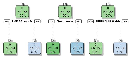
Each of these trees make their classification decisions based on different variables. So let’s imagine a female passenger from Southampton who rode in first class. Tree one and two would vote that she survived, but tree three votes that she perishes. If we take a vote, it’s 2 to 1 in favour of her survival, so we would classify this passenger as a survivor.

Random Forest models grow trees much deeper than the decision stumps above, in fact the default behaviour is to grow each tree out as far as possible, like the overfitting tree we made in lesson three. But since the formulas for building a single decision tree are the same every time, some source of randomness is required to make these trees different from one another. Random Forests do this in two ways.

The first trick is to use bagging, for bootstrap aggregating. Bagging takes a randomized sample of the rows in your training set, with replacement. This is easy to simulate in R using the sample function. Let’s say we wanted to perform bagging on a training set with 10 rows.

> sample(1:10, replace = TRUE)
 [1]  3  1  9  1  7 10 10  2  2  9

In this simulation, we would still have 10 rows to work with, but rows 1, 2, 9 and 10 are each repeated twice, while rows 4, 5, 6 and 8 are excluded. If you run this command again, you will get a different sample of rows each time. On average, around 37% of the rows will be left out of the bootstrapped sample. With these repeated and omitted rows, each decision tree grown with bagging would evolve slightly differently. If you have very strong features such as gender in our example though, that variable will probably still dominate the first decision in most of your trees.

The second source of randomness gets past this limitation though. Instead of looking at the entire pool of available variables, Random Forests take only a subset of them, typically the square root of the number available. In our case we have 10 variables, so using a subset of three variables would be reasonable. The selection of available variables is changed for each and every node in the decision trees. This way, many of the trees won’t even have the gender variable available at the first split, and might not even see it until several nodes deep.

Through these two sources of randomness, the ensemble contains a collection of totally unique trees which all make their classifications differently. As with our simple example, each tree is called to make a classification for a given passenger, the votes are tallied (with perhaps many hundreds, or thousands of trees) and the majority decision is chosen. Since each tree is grown out fully, they each overfit, but in different ways. Thus the mistakes one makes will be averaged out over them all.

R’s Random Forest algorithm has a few restrictions that we did not have with our decision trees. The big one has been the elephant in the room until now, we have to clean up the missing values in our dataset. rpart has a great advantage in that it can use surrogate variables when it encounters an NA value. In our dataset there are a lot of age values missing. If any of our decision trees split on age, the tree would search for another variable that split in a similar way to age, and use them instead. Random Forests cannot do this, so we need to find a way to manually replace these values.

A method we implicitly used in part 2 when we defined the adult/child age buckets was to assume that all missing values were the mean or median of the remaining data. Since then we’ve learned a lot of new skills though, so let’s use a decision tree to fill in those values instead. Let’s pick up where we left off last lesson, and take a look at the combined dataframe’s age variable to see what we’re up against:

> summary(combi$Age)
   Min. 1st Qu.  Median    Mean 3rd Qu.    Max.    NA's
   0.17   21.00   28.00   29.88   39.00   80.00     263

263 values out of 1309 were missing this whole time, that’s a whopping 20%! A few new pieces of syntax to use. Instead of subsetting by boolean logic, we can use the R function is.na(), and it’s reciprocal !is.na() (the bang symbol represents “not”). This subsets on whether a value is missing or not. We now also want to use the method="anova" version of our decision tree, as we are not trying to predict a category any more, but a continuous variable. So let’s grow a tree on the subset of the data with the age values available, and then replace those that are missing:

> Agefit <- rpart(Age ~ Pclass + Sex + SibSp + Parch + Fare + Embarked + Title + FamilySize,
                  data=combi[!is.na(combi$Age),], 
                  method="anova")
> combi$Age[is.na(combi$Age)] <- predict(Agefit, combi[is.na(combi$Age),])

I left off the family size and family IDs here as I didn’t think they’d have much impact on predicting age. You can go ahead and inspect the summary again, all those NA values are gone.

Let’s take a look at the summary of the entire dataset now to see if there are any other problem variables that we hadn’t noticed before:

> summary(combi)

Two jump out as a problem, though no where near as bad as Age, Embarked and Fare both are lacking values in two different ways.

> summary(combi$Embarked)
      C   Q   S
  2 270 123 914

Embarked has a blank for two passengers. While a blank wouldn’t be a problem for our model like an NA would be, since we’re cleaning anyhow, let’s get rid of it. Because it’s so few observations and such a large majority boarded in Southampton, let’s just replace those two with “S”. First we need to find out who they are though! We can use which for this:

> which(combi$Embarked == '')
[1]  62 830

This gives us the indexes of the blank fields. Then we simply replace those two, and encode it as a factor:

> combi$Embarked[c(62,830)] = "S"
> combi$Embarked <- factor(combi$Embarked)

The other naughty variable was Fare, let’s take a look:

> summary(combi$Fare)
   Min. 1st Qu.  Median    Mean 3rd Qu.    Max.    NA's
  0.000   7.896  14.450  33.300  31.280 512.300       1

It’s only one passenger with a NA, so let’s find out which one it is and replace it with the median fare:

> which(is.na(combi$Fare))
[1] 1044
> combi$Fare[1044] <- median(combi$Fare, na.rm=TRUE)

Okay. Our dataframe is now cleared of NAs. Now on to restriction number two: Random Forests in R can only digest factors with up to 32 levels. Our FamilyID variable had almost double that. We could take two paths forward here, either change these levels to their underlying integers (using the unclass() function) and having the tree treat them as continuous variables, or manually reduce the number of levels to keep it under the threshold.

Let’s take the second approach. To do this we’ll copy the FamilyID column to a new variable, FamilyID2, and then convert it from a factor back into a character string with as.character(). We can then increase our cut-off to be a “Small” family from 2 to 3 people. Then we just convert it back to a factor and we’re done:

> combi$FamilyID2 <- combi$FamilyID
> combi$FamilyID2 <- as.character(combi$FamilyID2)
> combi$FamilyID2[combi$FamilySize <= 3] <- 'Small'
> combi$FamilyID2 <- factor(combi$FamilyID2)

Okay, we’re down to 22 levels so we’re good to split the test and train sets back up as we did last lesson and grow a Random Forest. Install and load the package randomForest:

> install.packages('randomForest')
> library(randomForest)

Because the process has the two sources of randomness that we discussed earlier, it is a good idea to set the random seed in R before you begin. This makes your results reproducible next time you load the code up, otherwise you can get different classifications for each run.

> set.seed(415)

The number inside isn’t important, you just need to ensure you use the same seed number each time so that the same random numbers are generated inside the Random Forest function.

Now we’re ready to run our model. The syntax is similar to decision trees, but there’s a few extra options.

> fit <- randomForest(as.factor(Survived) ~ Pclass + Sex + Age + SibSp + Parch + Fare +
                                            Embarked + Title + FamilySize + FamilyID2,
                      data=train, 
                      importance=TRUE, 
                      ntree=2000)

Instead of specifying method="class" as with rpart, we force the model to predict our classification by temporarily changing our target variable to a factor with only two levels using as.factor(). The importance=TRUE argument allows us to inspect variable importance as we’ll see, and the ntree argument specifies how many trees we want to grow.

If you were working with a larger dataset you may want to reduce the number of trees, at least for initial exploration, or restrict the complexity of each tree using nodesize as well as reduce the number of rows sampled with sampsize. You can also override the default number of variables to choose from with mtry, but the default is the square root of the total number available and that should work just fine. Since we only have a small dataset to play with, we can grow a large number of trees and not worry too much about their complexity, it will still run pretty fast.

So let’s look at what variables were important:

> varImpPlot(fit)

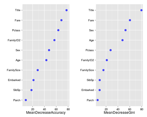
Remember with bagging how roughly 37% of our rows would be left out? Well Random Forests doesn’t just waste those “out-of-bag” (OOB) observations, it uses them to see how well each tree performs on unseen data. It’s almost like a bonus test set to determine your model’s performance on the fly.

There’s two types of importance measures shown above. The accuracy one tests to see how worse the model performs without each variable, so a high decrease in accuracy would be expected for very predictive variables. The Gini one digs into the mathematics behind decision trees, but essentially measures how pure the nodes are at the end of the tree. Again it tests to see the result if each variable is taken out and a high score means the variable was important.

Unsurprisingly, our Title variable was at the top for both measures. We should be pretty happy to see that the remaining engineered variables are doing quite nicely too. Anyhow, enough delay, let’s see how it did!

The prediction function works similarly to decision trees, and we can build our submission file in exactly the same way. It will take a bit longer though, as all 2000 trees need to make their classifications and then discuss who’s right:

> Prediction <- predict(fit, test)
> submit <- data.frame(PassengerId = test$PassengerId, Survived = Prediction)
> write.csv(submit, file = "firstforest.csv", row.names = FALSE)

Hrmm, well this actually worked out exactly the same as Kaggle’s Python random forest tutorial. I wouldn’t take that as the expected result from any forest though, this may just be pure coincidence. It’s relatively poor performance does go to show that on smaller datasets, sometimes a fancier model won’t beat a simple one. Besides that, there’s also the private leaderboard as only 50% of the test data is evaluated for our public scores.

But let’s not give up yet. There’s more than one ensemble model. Let’s try a forest of conditional inference trees. They make their decisions in slightly different ways, using a statistical test rather than a purity measure, but the basic construction of each tree is fairly similar.

So go ahead and install and load the party package.

> install.packages('party')
> library(party)

We again set the seed for consistent results and build a model in a similar way to our Random Forest:

> set.seed(415)
> fit <- cforest(as.factor(Survived) ~ Pclass + Sex + Age + SibSp + Parch + Fare +
                                       Embarked + Title + FamilySize + FamilyID,
                 data = train, 
                 controls=cforest_unbiased(ntree=2000, mtry=3))

Conditional inference trees are able to handle factors with more levels than Random Forests can, so let’s go back to out original version of FamilyID. You may have also noticed a few new arguments. Now we have to specify the number of trees inside a more complicated command, as arguments are passed to cforest differently. We also have to manually set the number of variables to sample at each node as the default of 5 is pretty high for our dataset. Okay, let’s make another prediction:

> Prediction <- predict(fit, test, OOB=TRUE, type = "response")

The prediction function requires a few extra nudges for conditional inference forests as you see. Let’s write a submission and submit it!

Congratulations! At the time of writing you are now in the top 5% of a Kaggle competition!

You’ve come a long way, from the bottom of the Kaggle leaderboard to the top! There may be a few more insights to wring from this dataset yet though. We never did look at the ticket or cabin numbers, so take a crack at extracting some insights from them to see if any more gains are possible. Maybe extracting the cabin letter (deck) or number (location) and extrapolating to the rest of the passengers’9 family if they’re missing might be worth a try?

While there’s just no way that I could introduce all the R syntax you’ll need to navigate dataframes in different situations, I hope that I’ve given you a good start. I linked to some good R guides way back in the introduction that should help you learn more, here and here, as well as an excellent book The Art of R Programming: A Tour of Statistical Software Design to continue learning about programming in R.

Well that’s it for the tutorial series. I really hope that you can exceed the benchmark I’ve posted here. If you find some new ideas that develop the base that I’ve presented, be sure to contribute back to the community through the Kaggle forums, or comment on the blog.

I hope you found the tutorials interesting and informative, and that they gave you a taste for machine learning that will spur you to compete in the prize-eligible Kaggle competitions! I hope to see you on the leaderboards out in the wild. Good luck and happy learning!

All code from this tutorial is available on my Github repository