Titanic: Getting Started With R - Part 4: Feature Engineering

Tutorial index

Feature engineering is so important to how your model performs, that even a simple model with great features can outperform a complicated algorithm with poor ones. In fact, feature engineering has been described as easily the most important factor in determining the success or failure of your predictive model. Feature engineering really boils down to the human element in machine learning. How much you understand the data, with your human intuition and creativity, can make the difference.

So what is feature engineering? It can mean many things to different problems, but in the Titanic competition it could mean chopping, and combining different attributes that we were given by the good folks at Kaggle to squeeze a little bit more value from them. In general, an engineered feature may be easier for a machine learning algorithm to digest and make rules from than the variables it was derived from.

The initial suspects for gaining more machine learning mojo from are the three text fields that we never sent into our decision trees last time. While the ticket number, cabin, and name were all unique to each passenger; perhaps parts of those text strings could be extracted to build a new predictive attribute. Let’s start with the name field. If we take a glance at the first passenger’s name we see the following:

> train$Name[1]
[1] Braund, Mr. Owen Harris
891 Levels: Abbing, Mr. Anthony Abbott, Mr. Rossmore Edward ... Zimmerman, Mr. Leo

Previously we have only accessed passenger groups by subsetting, now we access an individual by using the row number, 1, as an index instead. Okay, no one else on the boat had that name, that’s pretty much certain, but what else might they have shared? Well, I’m sure there were plenty of Mr’s aboard. Perhaps the persons title might give us a little more insight.

If we scroll through the dataset we see many more titles including Miss, Mrs, Master, and even the Countess! The title “Master” is a bit outdated now, but back in these days, it was reserved for unmarried boys. Additionally, the nobility such as our Countess would probably act differently to the lowly proletariat too. There seems to be a fair few possibilities of patterns in this that may dig deeper than the combinations of age, gender, etc that we looked at before.

In order to extract these titles to make new variables, we’ll need to perform the same actions on both the training and testing set, so that the features are available for growing our decision trees, and making predictions on the unseen testing data. An easy way to perform the same processes on both datasets at the same time is to merge them. In R we can use rbind, which stands for row bind, so long as both dataframes have the same columns as each other. Since we obviously lack the Survived column in our test set, let’s create one full of missing values (NAs) and then row bind the two datasets together:

> test$Survived <- NA
> combi <- rbind(train, test)

Now we have a new dataframe called “combi” with all the same rows as the original two datasets, stacked in the order in which we specified: train first, and test second.

If you look back at the output of our inquiry on Owen, his name is still encoded as a factor. As we mentioned earlier in the tutorial series, strings are automatically imported as factors in R, even if it doesn’t make sense. So we need to cast this column back into a text string. To do this we use as.character. Let’s do this and then take another look at Owen:

> combi$Name <- as.character(combi$Name)
> combi$Name[1]
[1] "Braund, Mr. Owen Harris"

Excellent, no more levels, now it’s just pure text. In order to break apart a string, we need some hooks to tell the program to look for. Nicely, we see that there is a comma right after the person’s last name, and a full stop after their title. We can easily use the function strsplit, which stands for string split, to break apart our original name over these two symbols. Let’s try it out on Mr. Braund:

> strsplit(combi$Name[1], split='[,.]')
[[1]]
[1] "Braund"       " Mr"          " Owen Harris"

Okay, good. Here we have sent strsplit the cell of interest, and given it some symbols to chose from when splitting the string up, either a comma or period. Those symbols in the square brackets are called regular expressions, though this is a very simple one, and if you plan on working with a lot of text I would certainly recommend getting used to using them!

We see that the title has been broken out on its own, though there’s a strange space before it begins because the comma occurred at the end of the surname. But how do we get to that title piece and clear out the rest of the stuff we don’t want? An index [[1]] is printed before the text portions. Let’s try to dig into this new type of container by appending all those square brackets to the original command:

> strsplit(combi$Name[1], split='[,.]')[[1]]
[1] "Braund"       " Mr"          " Owen Harris"

Getting there! String split uses a doubly stacked matrix because it can never be sure that a given regex will have the same number of pieces. If there were more commas or periods in the name, it would create more segments, so it hides them a level deeper to maintain the rectangular types of containers that we are used to in things like spreadsheets, or now dataframes! Let’s go a level deeper into the indexing mess and extract the title. It’s the second item in this nested list, so let’s dig in to index number 2 of this new container:

> strsplit(combi$Name[1], split='[,.]')[[1]][2]
[1] " Mr"

Great. We have isolated the title we wanted at last. But how to apply this transformation to every row of the combined train/test dataframe? Luckily, R has some extremely useful functions that apply more complicated functions one row at a time. As we had to dig into this container to get the title, simply trying to run combi$Title <- strsplit(combi$Name, split='[,.]')[[1]][2] over the whole name vector would result in all of our rows having the same value of Mr., so we need to work a bit harder. Unsurprisingly applying a function to a lot of cells in a dataframe or vector uses the apply suite of functions of R:

> combi$Title <- sapply(combi$Name, FUN=function(x) {strsplit(x, split='[,.]')[[1]][2]})

R’s apply functions all work in slightly different ways, but sapply will work great here. We feed sapply our vector of names and our function that we just came up with. It runs through the rows of the vector of names, and sends each name to the function. The results of all these string splits are all combined up into a vector as output from the sapply function, which we then store to a new column in our original dataframe, called Title.

Finally, we may wish to strip off those spaces from the beginning of the titles. Here we can just substitute the first occurrence of a space with nothing. We can use sub for this (gsub would replace all spaces, poor “the Countess” would look strange then though):

> combi$Title <- sub(' ', '', combi$Title)

Alright, we now have a nice new column of titles, let’s have a look at it:

> table(combi$Title)
        Capt          Col          Don         Dona           Dr     Jonkheer         Lady
           1            4            1            1            8            1            1
       Major       Master         Miss         Mlle          Mme           Mr          Mrs
           2           61          260            2            1          757          197
          Ms          Rev          Sir the Countess
           2            8            1            1

Hmm, there are a few very rare titles in here that won’t give our model much to work with, so let’s combine a few of the most unusual ones. We’ll begin with the French. Mademoiselle and Madame are pretty similar (so long as you don’t mind offending) so let’s combine them into a single category:

> combi$Title[combi$Title %in% c('Mme', 'Mlle')] <- 'Mlle'

What have we done here? The %in% operator checks to see if a value is part of the vector we’re comparing it to. So here we are combining two titles, “Mme” and “Mlle”, into a new temporary vector using the c() operator and seeing if any of the existing titles in the entire Title column match either of them. We then replace any match with “Mlle”.

Let’s keep looking for redundancy. It seems the very rich are a bit of a problem for our set here too. For the men, we have a handful of titles that only one or two have been blessed with: Captain, Don, Major and Sir. All of these are either military titles, or rich fellas who were born with vast tracts of land.

For the ladies, we have Dona, Lady, Jonkheer (*see comments below), and of course our Countess. All of these are again the rich folks, and may have acted somewhat similarly due to their noble birth. Let’s combine these two groups and reduce the number of factor levels to something that a decision tree might make sense of:

> combi$Title[combi$Title %in% c('Capt', 'Don', 'Major', 'Sir')] <- 'Sir'
< combi$Title[combi$Title %in% c('Dona', 'Lady', 'the Countess', 'Jonkheer')] <- 'Lady'

Our final step is to change the variable type back to a factor, as these are essentially categories that we have created:

> combi$Title <- factor(combi$Title)

Alright. We’re done with the passenger’s title now. What else can we think up? Well, there’s those two variables SibSb and Parch that indicate the number of family members the passenger is travelling with. Seems reasonable to assume that a large family might have trouble tracking down little Johnny as they all scramble to get off the sinking ship, so let’s combine the two variables into a new one, FamilySize:

> combi$FamilySize <- combi$SibSp + combi$Parch + 1

Pretty simple! We just add the number of siblings, spouses, parents and children the passenger had with them, and plus one for their own existence of course, and have a new variable indicating the size of the family they travelled with.

Anything more? Well we just thought about a large family having issues getting to lifeboats together, but maybe specific families had more trouble than others? We could try to extract the Surname of the passengers and group them to find families, but a common last name such as Johnson might have a few extra non-related people aboard. In fact there are three Johnsons in a family with size 3, and another three probably unrelated Johnsons all travelling solo.

Combining the Surname with the family size though should remedy this concern. No two family-Johnson’s should have the same FamilySize variable on such a small ship. So let’s first extract the passengers’ last names. This should be a pretty simple change from the title extraction code we ran earlier, now we just want the first part of the strsplit output:

> combi$Surname <- sapply(combi$Name, FUN=function(x) {strsplit(x, split='[,.]')[[1]][1]})

We then want to append the FamilySize variable to the front of it, but as we saw with factors, string operations need strings. So let’s convert the FamilySize variable temporarily to a string and combine it with the Surname to get our new FamilyID variable:

combi$FamilyID <- paste(as.character(combi$FamilySize), combi$Surname, sep="")

We used the function paste to bring two strings together, and told it to separate them with nothing through the sep argument. This was stored to a new column called FamilyID. But those three single Johnsons would all have the same Family ID. Given we were originally hypothesising that large families might have trouble sticking together in the panic, let’s knock out any family size of two or less and call it a “small” family. This would fix the Johnson problem too.

> combi$FamilyID[combi$FamilySize <= 2] <- 'Small'

Let’s see how we did for identifying these family groups:

> table(combi$FamilyID)
           11Sage           3Abbott         3Appleton         3Beckwith           3Boulos
               11                 3                 1                 2                 3
          3Bourke            3Brown         3Caldwell          3Christy          3Collyer
                3                 4                 3                 2                 3
         3Compton          3Cornell           3Coutts           3Crosby           3Danbom
                3                 1                 3                 3                 3 . . .

Hmm, a few seemed to have slipped through the cracks here. There’s plenty of FamilyIDs with only one or two members, even though we wanted only family sizes of 3 or more. Perhaps some families had different last names, but whatever the case, all these one or two people groups is what we sought to avoid with the three person cut-off. Let’s begin to clean this up:

> famIDs <- data.frame(table(combi$FamilyID))

Now we have stored the table above to a dataframe. Yep, you can store most tables to a dataframe if you want to, so let’s take a look at it by clicking on it in the explorer:

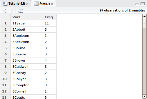
Here we see again all those naughty families that didn’t work well with our assumptions, so let’s subset this dataframe to show only those unexpectedly small FamilyID groups.

famIDs <- famIDs[famIDs$Freq <= 2,]

We then need to overwrite any family IDs in our dataset for groups that were not correctly identified and finally convert it to a factor:

> combi$FamilyID[combi$FamilyID %in% famIDs$Var1] <- 'Small'
> combi$FamilyID <- factor(combi$FamilyID)

We are now ready to split the test and training sets back into their original states, carrying our fancy new engineered variables with them. The nicest part of what we just did is how the factors are treated in R. Behind the scenes, factors are basically stored as integers, but masked with their text names for us to look at. If you create the above factors on the isolated test and train sets separately, there is no guarantee that both groups exist in both sets.

For instance, the family “3Johnson” previously discussed does not exist in the test set. We know that all three of them survive from the training set data. If we had built our factors in isolation, there would be no factor “3Johnson” for the test set. This would upset any machine learning model because the factors between the training set used to build the model and the test set it is asked to predict for are not consistent. ie. R will throw errors at you if you try.

Because we built the factors on a single dataframe, and then split it apart after we built them, R will give all factor levels to both new dataframes, even if the factor doesn’t exist in one. It will still have the factor level, but no actual observations of it in the set. Neat trick right? Let me assure you that manually updating factor levels is a pain.

So let’s break them apart and do some predictions on our new fancy engineered variables:

> train <- combi[1:891,]
> test <- combi[892:1309,]

Here we introduce yet another subsetting method in R; there are many depending on how you want to chop up your data. We have isolated certain ranges of rows of the combi dataset based on the sizes of the original train and test sets. The comma after that with no numbers following it indicates that we want to take ALL columns with this subset and store it to the assigned dataframe. This gives us back our original number of rows, as well as all our new variables including the consistent factor levels.

Time to do our predictions! We have a bunch of new variables, so let’s send them to a new decision tree. Last time the default complexity worked out pretty well, so let’s just grow a tree with the vanilla controls and see what it can do:

> fit <- rpart(Survived ~ Pclass + Sex + Age + SibSp + Parch + Fare + Embarked + Title + FamilySize + FamilyID,
               data=train, 
               method="class")

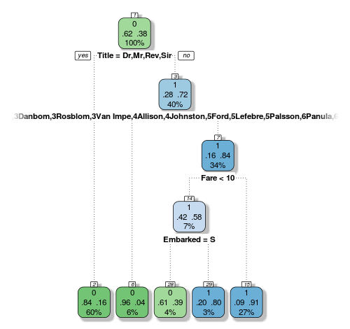
Interestingly our new variables are basically governing our tree. Here’s another drawback with decision trees that I didn’t mention last time: they are biased to favour factors with many levels. Look at how our 61-level FamilyID factor is so prominent here, and the tree picked out all the families that are biased one way more than the others. This way the decision node can chop and change the data into the best way possible combination for purity of the following nodes.

But all that aside, you know should know how to create a submission from a decision tree, so let’s see how it performed!

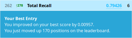
Awesome, we just almost halved our rank! All by squeezing a bit more value out of what we already had. And this is just a sample of what you might be able to find in this dataset.

Go ahead and try and create some more engineered variables! As before, I also really encourage you to play around with the complexity parameters and maybe try trimming some deeper trees to see if it helps or hinders your rank. You may even consider excluding some variables from the tree to see if that changes anything too.

In most cases though, the title or gender variables will govern the first decision due to the greedy nature of decision trees. The bias towards many-levelled factors won’t go away either, and the overfitting problem can be difficult to gauge without actually sending in submissions, but good judgement can help.

Next lesson, we will overcome these limitations by building an ensemble of decision trees with the powerful Random Forest algorithm. Go there now!

All code from this tutorial is available on my Github repository